 Home
HomeCartogram Plotting Using R
A cartogram is a thematic map where a certain mapping variable (e.g., population or economic indicator) of a geographic region is substituted for its physical (land) area. The spatial geometry of the map is then proportionately distorted in order to reflect the information conveyed by the thematic variable. Cartograms are thus visually intuitive and revealing to the presentation of such information.
There exist a few algorithms to compute cartograms given the land densities and thematic variables. One of them is the diffusion-based method proposed by Gatsner and Newman, in which the authors also provide a neat C program to compute the point-wise cartogram transformations. Check out some of the very revealing maps extracted from their book Atlas of the Real World.
This post demonstrates how to compute and plot cartograms using R and given input shapefiles by interfacing with the above-mentioned C program via two packages: Rcartogram and getcartr. I was first motivated by this post, in which the author did not find an easy way to make cartograms using R and resorted to using the off-the-shelf tool ScapeToad. In this blog post, I will show how to plot the cartogram of the world’s population by country in 2013, whose data can be downloaded here.
All the source code in this tutorial can be downloaded from this GitHub repo.
Preparations
First, make sure you have the two packages FFTW3 and “fftw” for R, which perform fast Fourier transform, properly installed. For Linux and macOS, do the following (courtesy of this article):
- Download the latest FFTW package.
- Extract to a directory and
cdthere. - On the Terminal, type:
./configure --enable-shared - Then compile the package:
make, and install it:sudo make install
If nothing goes wrong, the library should be correctly installed. Now, download fftw to some directory. In that directory, type: sudo R CMD INSTALL fftw_1.0-3.tar.gz, where fftw_1.0-3.tar.gz is the name of the downloaded file. This would compile and install the R package.
The next steps are to be performed in an R environment (e.g., RStudio). We are now going to install two R packages from GitHub: Rcartogram and getcartr. (Thus, make sure you have devtools package installed.) The former bundles the compiled C binaries with some neat R functions to interface with them. Whereas, the latter provides a means to interface with Rcartogram and the C library through which the input shapefile and its carto-transformed polygons can be effectively plotted.
library(devtools)
install_github('omegahat/Rcartogram')
## Wait for installation, then:
install_github('chrisbrunsdon/getcartr', subdir='getcartr')
Finally, make sure you have ggplot2, maptools, and rgeos properly installed in R for geospatial visualization and data manipulations. (The last two are required for getcartr, anyways.)
Loading packages and data
First, load all the necessary packages at the beginning of your script:
library(Rcartogram)
library(getcartr)
library(ggplot2)
Then, read the shapefile that contains the map that you wish to plot. In this case, it is the world map with country borders. The corresponding shapefile can be downloaded from here.
world <- readShapePoly('TM_WORLD_BORDERS-0.3.shp')Next, read the data frame that contains the thematic variable of interest. In this example, it is the world’s population by country in 2013. This means the shape and size of each country (and respective boundaries) will be transformed and distorted proportionally to its population (and land area).
## We are using the world's population data from World Bank
world.pop <- read.csv(file = 'sp.pop.totl_Indicator_en_csv_v2.csv', stringsAsFactors = FALSE)
## Create a smaller dataset by retaining the world's population in 2013 and the ISO3
## country code, which will be used for matching and merging with the input shapefile
smaller.data <- data.frame(Country.Code = world.pop$Country.Code, Population = world.pop$X2013)
smaller.data <- na.omit(smaller.data)
Combining data and plotting the cartogram
In this last step, we will first join the two datasets world and smaller.data by their common field: ISO3 and Country.Code, respectively. We then compute the cartogram transformations of all the density points that make up the areas of all the countries according to their populations using the quick.carto function. (ISO3 code is a 3-letter representation of all the countries in the world.)
## Join the two datasets using their common field
matched.indices <- match(world@data[, "ISO3"], smaller.data[, "Country.Code"])
world@data <- data.frame(world@data, smaller.data[matched.indices, ])
## Compute the cartogram transformation of each country using its population
## with the degree of Gaussian blur = 0.5 (otherwise, it may not work)
world.carto <- quick.carto(world, world@data$Population, blur = 0.5)
In order to plot the resulted cartogram, we need to convert world.carto into a plottable data frame. The data frame will then be merged with the input shapefile using their shared field Country.Code.
## Convert the object into data frame
world.f <- fortify(world.carto, region = "Country.Code")
## Merge the cartogram transformation with the world map shapefile
world.f <- merge(world.f, world@data, by.x = "id", by.y = "Country.Code")
## Make a plot of the transformed polygons, where each country is
## further shaded by their population size (lighter means bigger)
my_map <- ggplot(world.f, aes(long, lat, group = group, fill = world.f$Population)) + geom_polygon()
## Display the plot and give it a title
(my_map <- my_map + ggtitle("Cartogram of the World Population (2013)"))
Finally, this is the cartogram we wish to see:
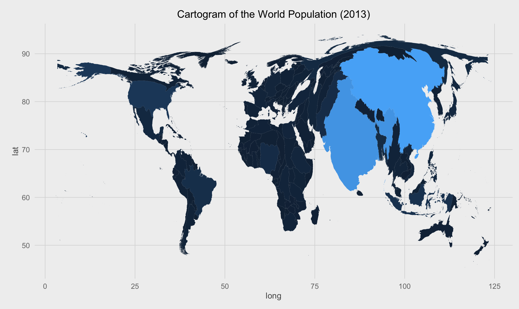
Compare this with the conventional thematic map and see the difference in how much more visual information a cartogram can convey!
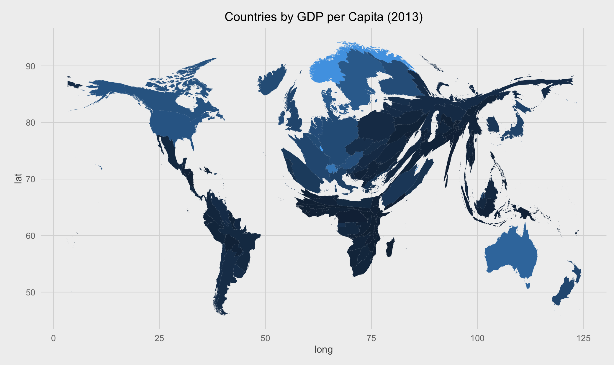
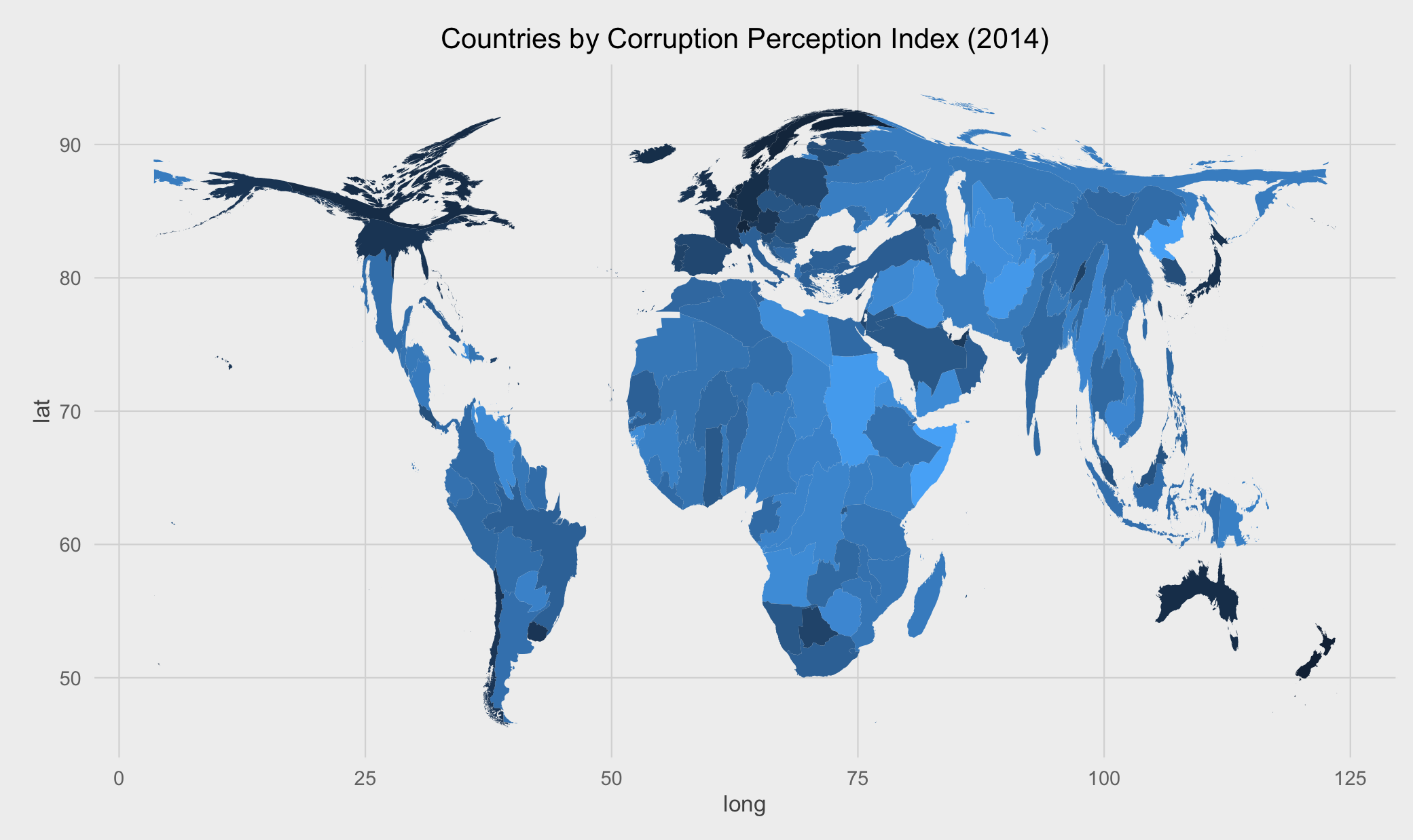
Here are other two revealing cartograms: world countries by GDP per capita (2013) and the Corruption Perception Index (2014), respectively.