Name Matching Model for Entity Resolution (Part 2)

This is Part II of a two-part series; for Part I, click here.

This post follows up on the previous one to demonstrate a practical application of the Name Matching model, namely entity resolution for transaction monitoring (TM).

In transaction monitoring, entity resolution (ER) is the problem of determining whether two different records (such as beneficiaries) refer to the same real-world entity (person or organization). Banks and payment platforms often ingest data from multiple sources, each with its own format, language and error pattern. Without robust ER, the same individual may appear as several distinct entities, fragmenting risk signals and weakening downstream controls.

This challenge is especially acute in AML and fraud detection, where TM systems rely on aggregating behaviors over time and across accounts. If transactions linked to the same underlying entity are split across multiple profiles, suspicious patterns such as structuring and rapid movements may remain undetected. On the other hand, overly aggressive matching can incorrectly merge truly distinct individuals, leading to false positives and unnecessary investigations.

Consider an individual who appears in different records as: Michael Lim, Mike Lim and Mr. Liem, Michael, a naive exact-match would treat these as three separate entities. Effective ER combines multiple signals (string similarity, token overlap, phonetic resemblance, etc.) to infer that these records likely refer to the same real-world person. Once resolved, all associated transactions can be analyzed holistically, enabling more accurate risk scoring.

For a more comprehensive introduction to ER, refer to this blog post. The following sections elaborate on how Name Matching can be incorporated into an effective ER pipeline for transaction monitoring with a hypothetical, yet realistic working example.

Entity resolution pipeline

The figure below illustrates a simple, yet effective ER pipeline for TM using Name Matching.

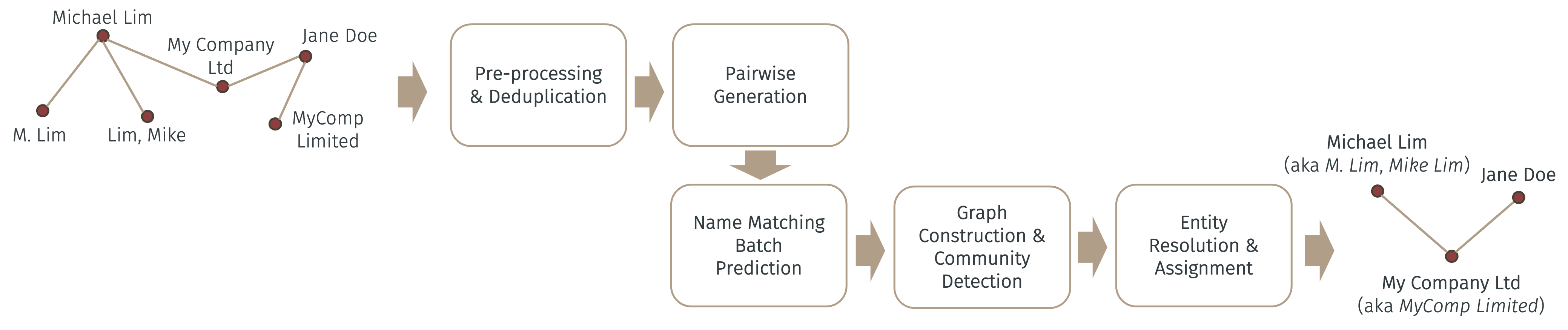
As illustrated above, name strings are first pre-processed (i.e., upper-cased, removed non-ASCII characters, numbers and punctuations) and deduplicated post pre-processing. The simple string deduplication step is to “match” names that only differ by simple characters or punctuations (such as John Doe and John, DOE) as the first cut.

The next step is to generate all pairwise comparisons of the names to be matched – called “candidates”. This is because Name Matching works by comparing a pair of names (name_x and name_y) at a time. Since there are O(n²) such pairs (where n is the number of names left after deduplication), the benefit of the previous deduplication step should be obvious now.

Suppose all name pairs form a data frame with name_x and name_y as columns. This data frame can then be batch predicted (for better efficiency) using the batch prediction API of Name Matching – refer to the API documentation for details. The result of which is another column that gives the probability of each pair of names (row) being matched. Depending on the chosen threshold (e.g., 0.85), any pair whose probability exceeds such threshold is considered a match.

After this, suppose a matched pair forms an edge in a graph such that we can construct an undirected graph from all matched pairs. This can be done using the NetworkX package. The purpose of this is to detect close-knit “communities” of nodes, where each node is a name, such that each community represents a resolved entity. The idea is that if pairs of names are so closely matched that they form a close-knit community in a graph, they can be also considered a real-world entity by this merit. An extreme version of which is a clique or a complete subgraph. There are many community detection algorithms on graphs – and the one implemented here is the popular Louvain method.

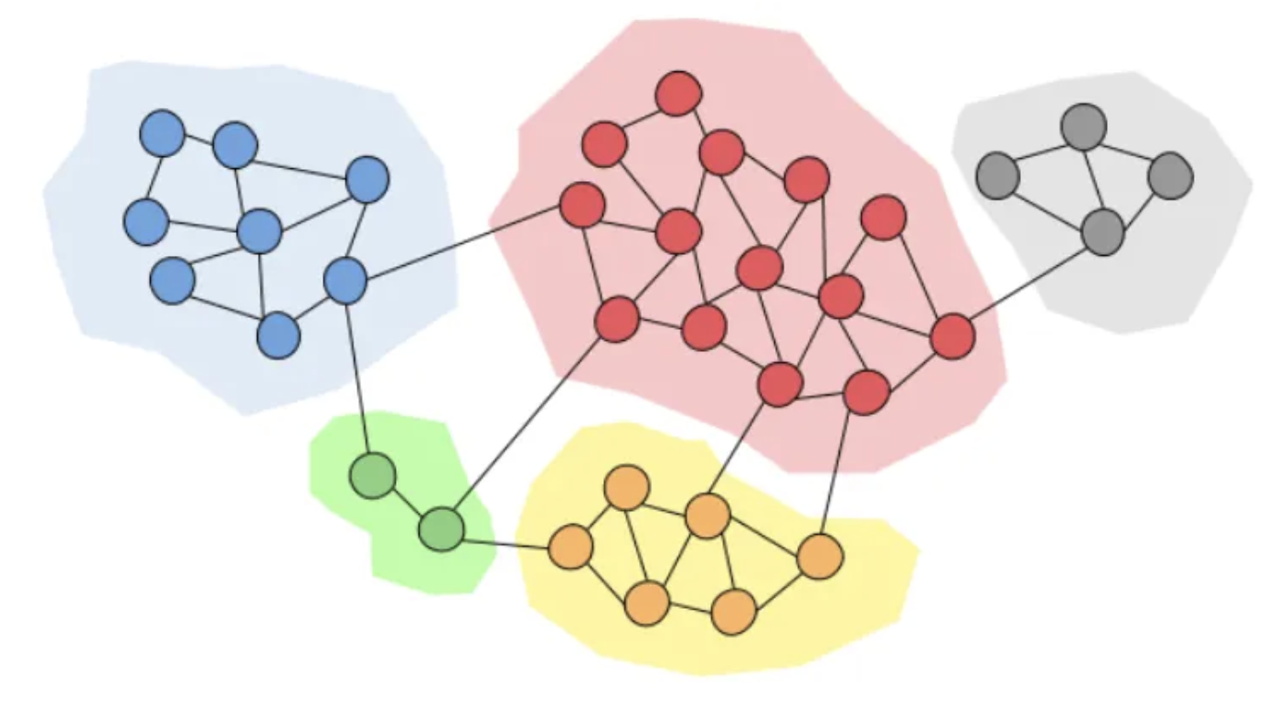
The figure below illustrates the concept of communities in a graph, where each community (represented by a distinct color) can be considered a resolved entity.

Finally, names in the original transactions are “resolved” and assigned a common entity name if they belong to the same community. That is, if we model the original transactions as a graph, where each node is a name and each edge is a transactional relationship, previously separate nodes (names) can now be “merged” into one if they are determined to be similar enough – and likewise, their corresponding edges can also be combined. Therefore, this resolved transaction graph represents more accurately the true relationships of the entities involved.

Python code implementing this entire ER pipeline is located here. The next section illustrates this proposed solution more clearly with a realistic working example.

A worked example

Suppose we have a simple dataset of mockup transactions whose names are adopted from the John Wick franchise containing ten transactions. The graph of the original transactions is illustrated by the figure below.

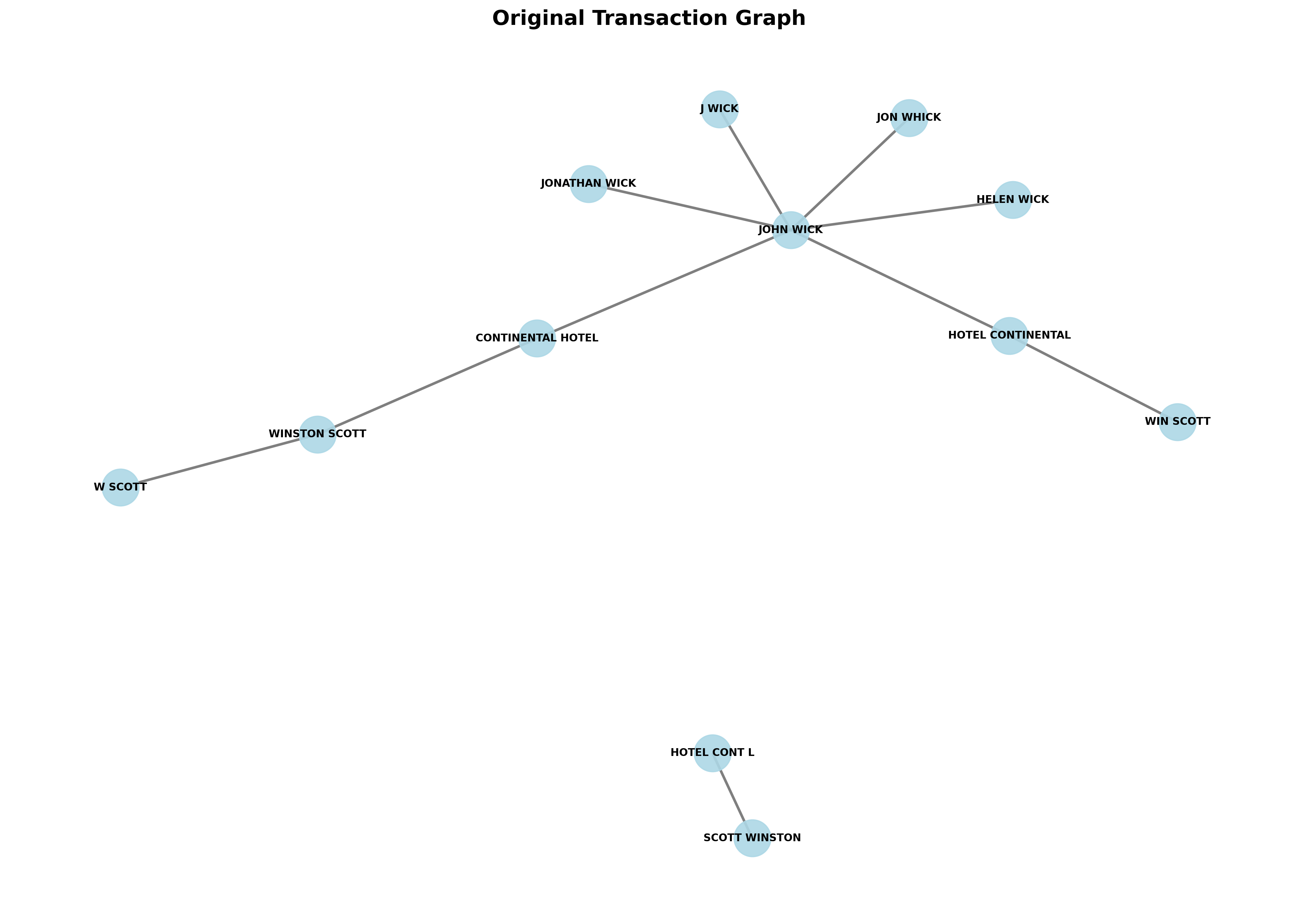
The graph shows the transactional relationships of all the names appearing in the dataset, where each unique name is a node and each transaction is an edge. It also shows, intuitively, that the following names very likely refer to the same underlying entities:

• John Wick, Jonathan Wick, J Wick and Jon Whick
• Continental Hotel, Hotel Continental and Hotel Cont'l
• Winston Scott, W Scott, Scott Winston and Win Scott

Note that entities such as Continental Hotel and Hotel Cont'l don’t need to have any (direct or indirect) transactional relationship with each other in order to be resolved. This is clearly shown in the graph as they belong to two distinct connected components. They can still be resolved, however, thanks to the all pairwise comparisons step of the pipeline as described above.

If we run the proposed ER pipeline on this dataset, we would obtain the following resolved graph.

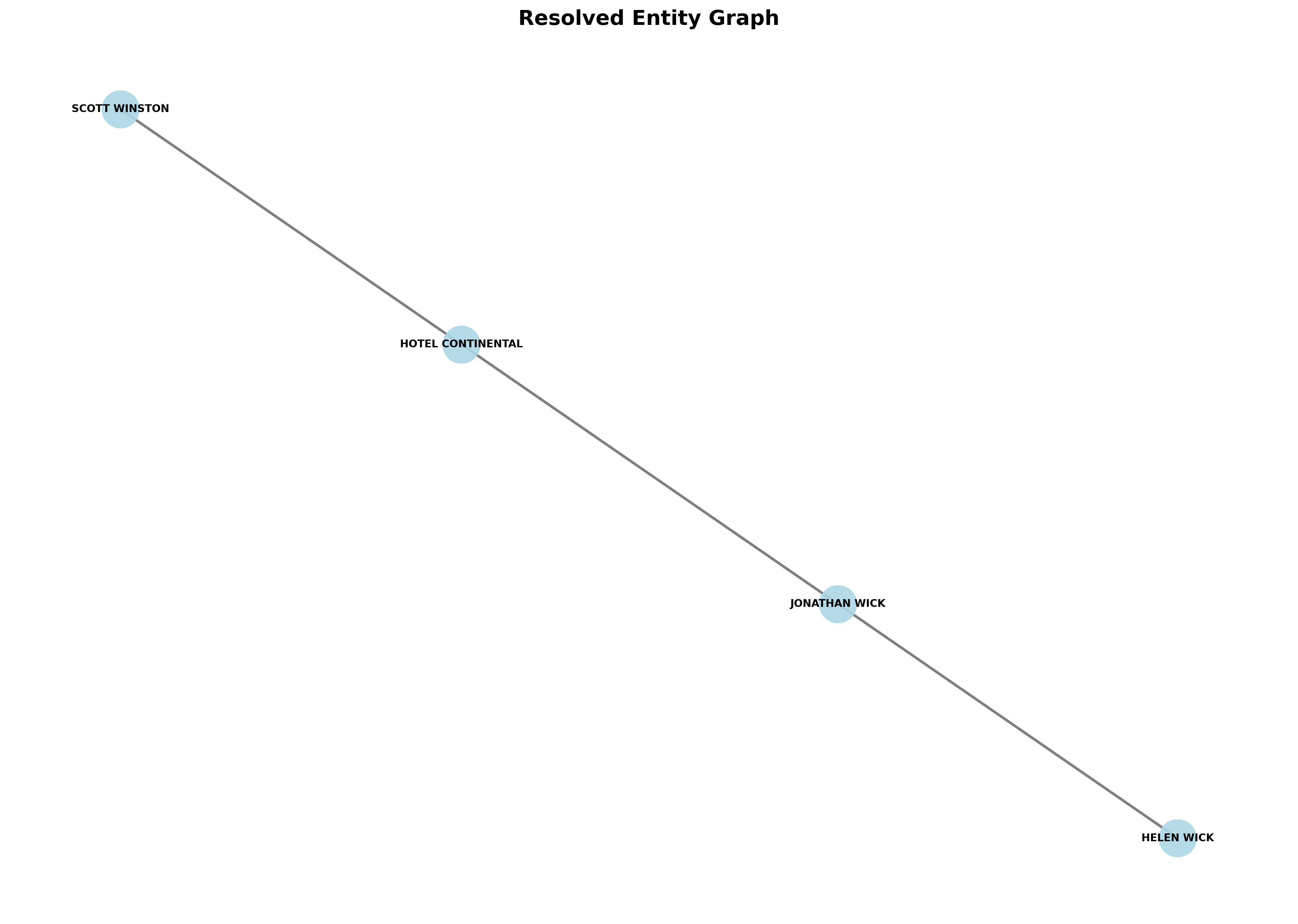
As expected, aliases of the same entity (as inferred by the model given some chosen threshold) are merged into one, described by a common node (name). Transactional relationships (edges) of the merged nodes are also combined to create a much “cleaner” and less fragmented graph that captures more accurately the true transactional relationships among the resolved entities. The pipeline finally updates the original transaction dataset with the resolved entity names as its output.